


The figures below are the interactive versions of the figures in the article, in the article’s order and under the article’s numbers. Hover a series for its values, drag across a chart to zoom and double-click to reset, and click a legend entry to hide or isolate a series.
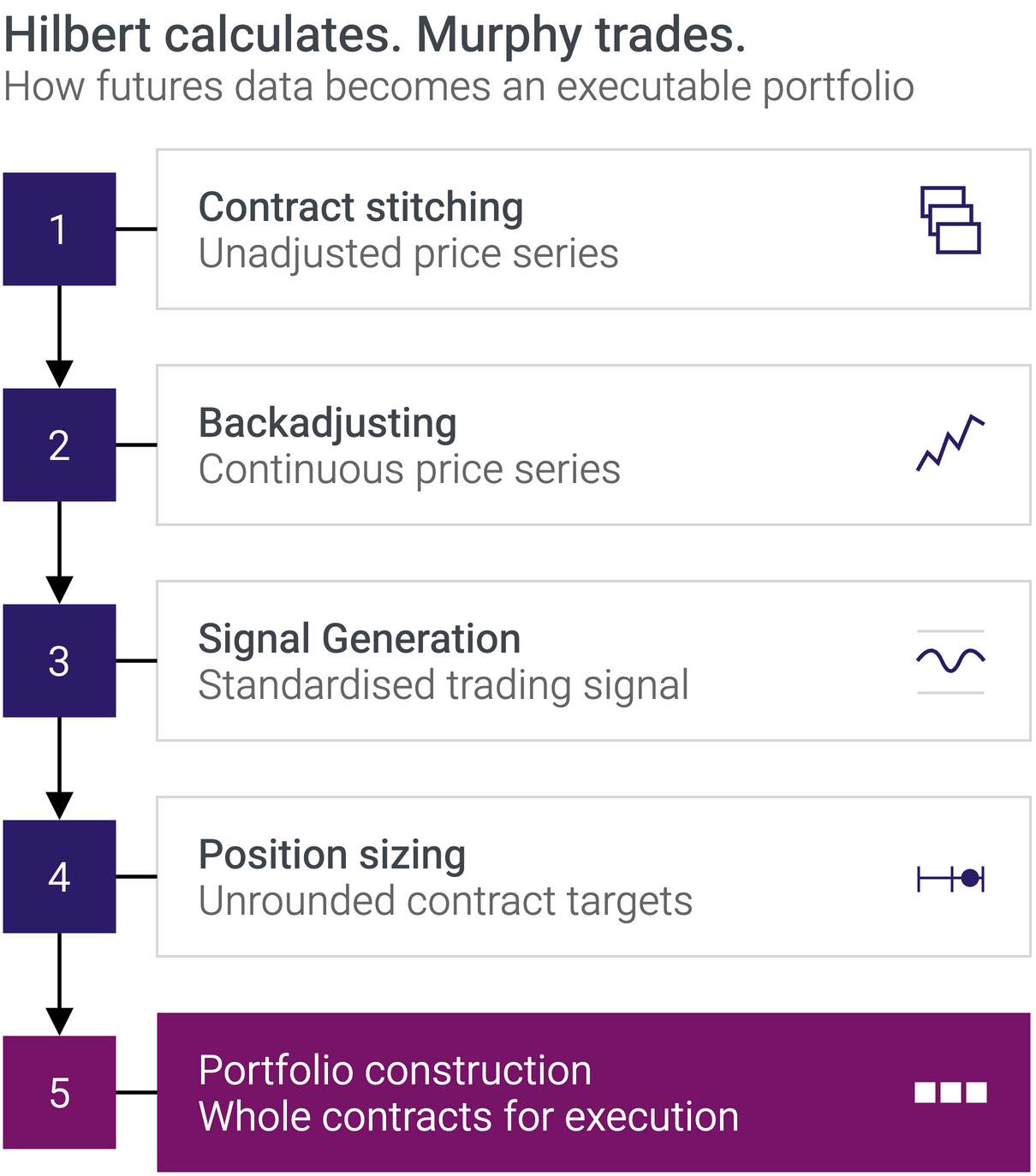
Figure 1. From contract histories to executable whole contracts.
Note: The final construction step also enforces position limits.
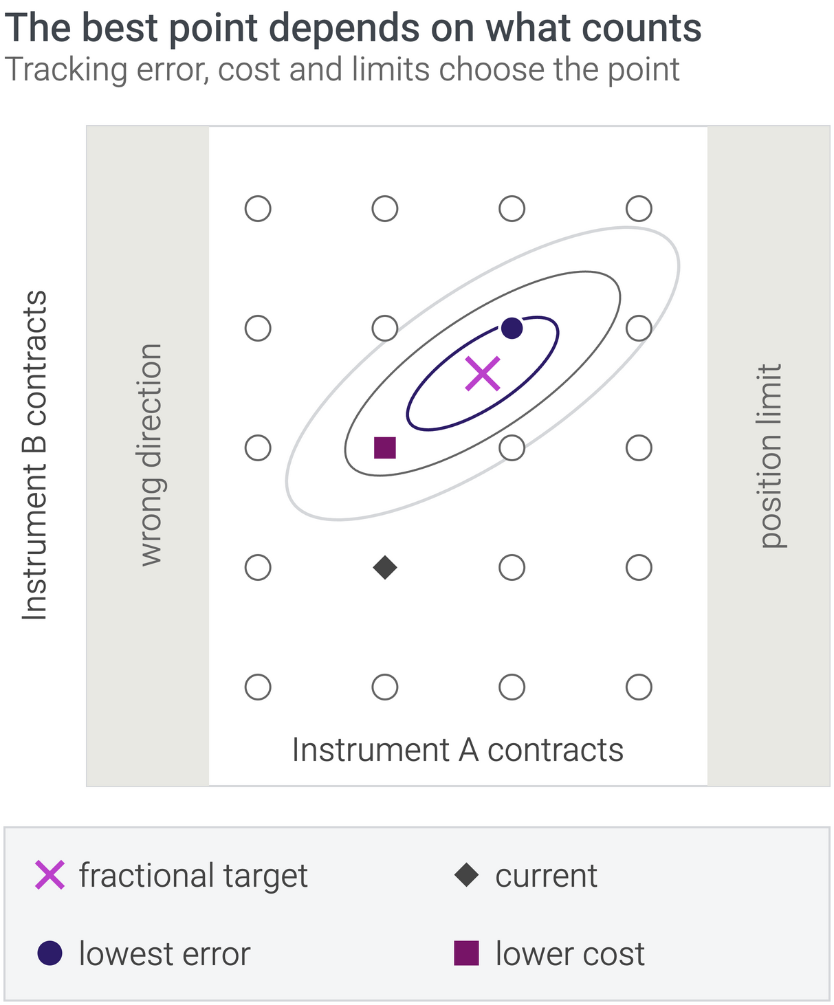
Figure 2. Each dot is an executable whole-contract portfolio. Contours show equal tracking error, while costs and limits choose the preferred point.
Note: Schematic two-instrument example.
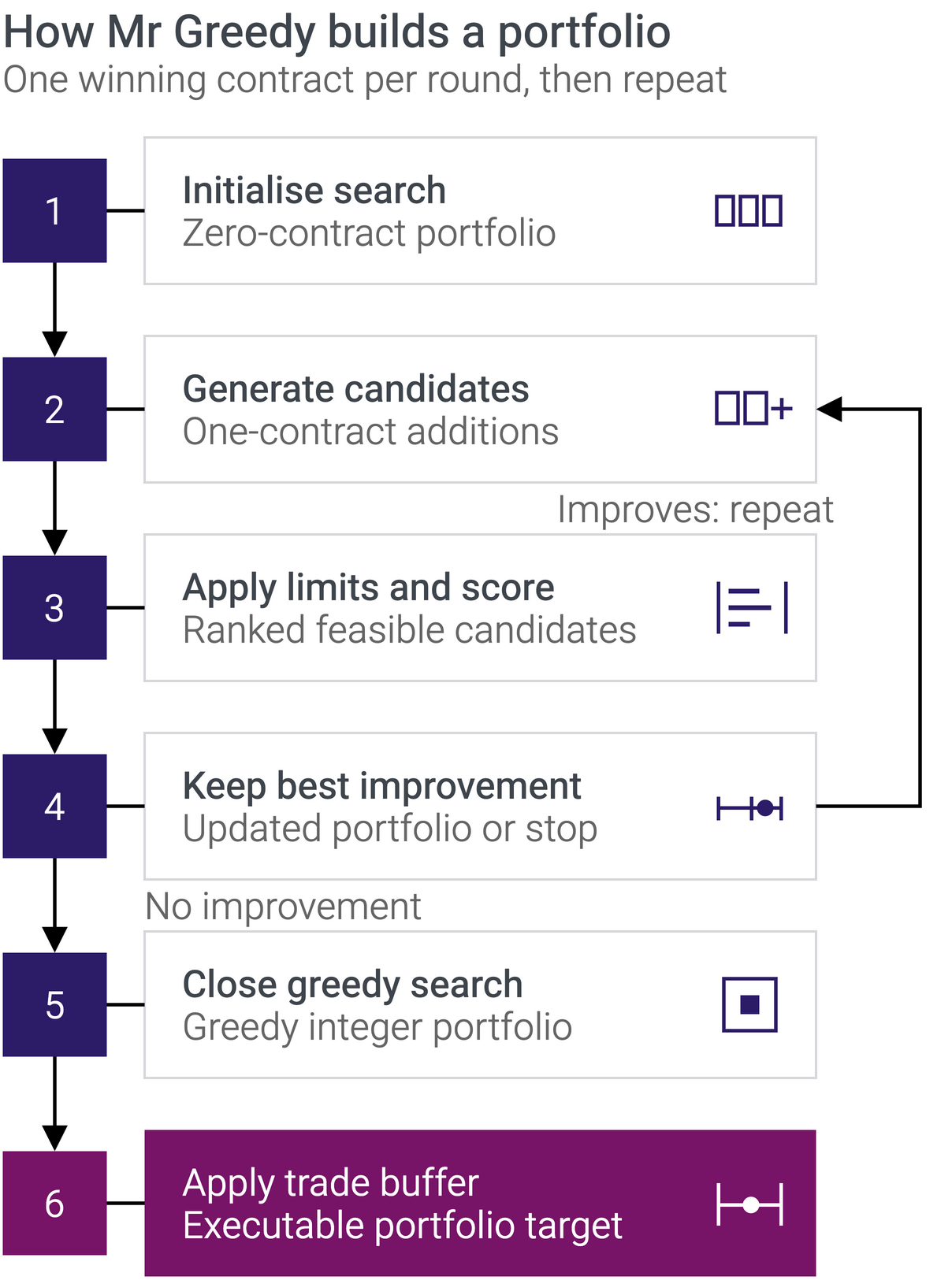
Figure 3. Each round keeps the legal one-contract candidate that lowers the objective most.
Note: The no-trade buffer is applied only after the greedy search has stopped.
Figure 4. SCIP tracks more closely in all nine experiments, and its advantage generally widens with capital.
Note: Strips show the small, medium and large portfolios. Greedy endpoints use lighter blue filled diamonds, and SCIP endpoints use darker blue filled circles. Values are predicted annualized tracking errors. Lower is better.
Figure 5. SCIP incurs lower costs than Greedy in eight of the nine experiments.
Note: Strips show the small, medium and large portfolios. Cost advantage equals Greedy minus SCIP in annualized percentage points. Positive values mean SCIP costs less.
Figure 6. SCIP gives up less after-cost Sharpe than Greedy in every experiment.
Note: Strips show the small, medium and large portfolios. Greedy uses lighter blue filled diamonds, and SCIP uses darker blue filled circles. Endpoint labels give each method’s after-cost Sharpe loss. Backtests begin on June 2, 1975, for the small portfolio and March 18, 1975, for the medium and large portfolios. All end on October 1, 2026. Values are Sharpe points. The unrounded benchmarks’ full-sample Sharpes are 1.50, 1.64, and 1.68, respectively, and each benchmark consists of a blend of divergence and convergence strategies.
Full textRead the complete article online · Figures omitted
Letter from the editor
For years, a greedy algorithm based on Rob Carver’s work turned my system’s ideal futures positions into orders for whole contracts. It is fast, transparent and proven in production. Nevertheless, I wanted to know how close its answer came to the optimum.
I expected a programming exercise. Instead, I found elegant portfolio-construction papers that stopped just before the practical difficulties began: transaction costs, changing position limits and hundreds of integer variables.
Translating the mathematics into a reliable program was harder. Covariance matrices had to remain well behaved. Results had to remain identical across different CPU architectures. A small change could determine whether the optimizer answered quickly or spent its time proving that a nearly identical answer could not be improved. “Optimal” did not automatically mean “safe to trade.”
Somewhere between the papers, source code and solver logs, my thinking split in two: the mathematician in me wanted the best answer. The engineer wanted something that would survive in production. So I gave them names.
Hilbert lives at the blackboard, where every problem yields to the correct formulation. He wants the global optimum and regards approximations as unfinished work. Murphy lives in production, where prices go missing, covariance matrices break and the best decision is worthless if it arrives too late. He wants an order the broker will accept.
Neither got the final word. Hilbert had to formulate an objective the solver could handle. Murphy had to make the result reproducible, fast and safe. The resulting procedure is their compromise: close enough to the mathematical ideal to preserve its intended risk profile, yet practical enough to survive in production. And it yielded better results!
The Question
How do you turn an ideal futures portfolio into whole-contract positions without losing the portfolio you designed?
The Answer
Define an objective that combines covariance-weighted tracking error and transaction costs, then solve it numerically.
- 0.06 higher Sharpe
- 0.5 pp lower annualized costs
- 3.4% tracking error
Hypothetical results. After-cost Sharpe includes estimated costs. See Appendix A.
Whether you are a diversified retail futures trader or manage a small hedge fund, you face the same dilemma. Hundreds of markets could diversify your portfolio, but your capital is limited.
One option is to trade a smaller set of futures. But that can leave you with regrets: what if you excluded heating oil in your last review and then missed its 2026 rally?
Another is to trade only those instruments with the strongest current signals. But selecting only extreme signals places too much confidence in noisy forecasts. It also leaves the underlying problem unsolved: what if too many instruments have strong signals and together require more capital than you have available?
Both choices sacrifice diversification and, typically, performance. But there is another approach.
Your trading system can generate continuous target positions for the full universe, even when it produces an untradable target such as 0.03 crude oil contracts. Portfolio construction then converts the ideal portfolio into whole-contract positions.
This means that you can trade even a big-boy portfolio of 301 instruments. I estimate that a naively rounded version would require roughly $500 million in capital for a full-strength target in the most capital-intensive instrument to reach at least four contracts.
The question is how to make that approximation without losing the diversification and risk profile you designed. This article will show you how.
Untradable Portfolio
The model wants 0.03 contracts. The broker insists on at least one.
Your trading system has done everything right: it has cleaned the data, generated a signal, allocated risk and calculated the position it wants. Then it asks you to buy 0.03 crude oil contracts.
That impossible order is where portfolio construction begins.
Before Hilbert reaches for the equations, Murphy points to the order ticket. The broker will accept one contract or none. It will not accept the mathematically elegant answer in between.
Figure 1 shows how an entirely sensible trading process produces this awkward result. Futures data begins as a collection of separate contract histories. In steps 1 and 2, the system joins successive expirations according to their roll schedules and back-adjusts prices across each roll. The result is one continuous price history for each instrument.
In step 3, each strategy converts that history into a bounded signal. I scale my signals from -20 to +20. Zero means no position, +10 represents a normal long position and +20 represents a strong long position. Negative values express the corresponding short positions. When several strategies trade the same instrument, I combine their individual signals so that they can share a single capital allocation.
Step 4 converts that signal into an ideal position. Available capital is distributed across asset classes and instruments, while risk and signal strength determine the desired exposure. The result is mathematically valid but not necessarily tradable. A target of 0.03 crude oil contracts is not a calculation error. It is the correct expression of the exposure the system wants at a given portfolio size.
An unrounded backtest therefore describes an ideal world: either contracts are divisible, or the provided capital is large enough for granularity to become negligible. This ideal portfolio is a useful benchmark, but it cannot be traded.
The obvious solution is to round every position to the nearest whole contract. Unfortunately, when a large futures universe is traded with only a few million dollars in capital, nearly every position would be rounded to zero.
Step 5 therefore considers the portfolio as a whole. It finds the whole-contract positions that best preserve the intended exposures within the account’s limits.
Hilbert sees an integer optimization problem. Murphy sees the orders needed before Tokyo opens.
Portfolio Construction Problem
Constructing tradable portfolios while controlling tracking error, costs and constraints.
Hilbert has calculated the perfect portfolio. It is diversified, risk-balanced and contains exactly 0.03 crude-oil contracts. Murphy looks at the order ticket. “That does not work.”
That disagreement is the portfolio construction problem. Hilbert wants the whole-contract portfolio that most closely reproduces the mathematical target. Murphy wants a portfolio that can actually be traded without wasting money on transaction costs, violating limits or creating risks that nobody intended.
They cannot both get everything they want, and even the name of the problem invites an argument.
The literature uses portfolio selection, portfolio optimization and portfolio construction for overlapping tasks. Markowitz called the original mean-variance problem portfolio selection1. Forecasts of future returns become a portfolio by balancing expected return against risk. Modern authors use portfolio construction2 for extensions of that framework, while closely related work calls the task portfolio optimization3.
Hilbert calls \(\epsilon\) the tracking error. Murphy calls it the list of compromises.
Solution requirements
An executable portfolio must respect trading costs, directional exposure and position limits. Closeness to its target is not enough.
I use portfolio construction for converting the unrounded portfolio into positions that can actually be traded. Portfolio optimization has another role in my system: it determines the proportions allocated to strategies or asset classes. Portfolio optimization will be the subject of a future article. Regular readers may now be thinking, “Not again! Every article announces at least five more articles!” Bear with me. We will eventually get there.
Hilbert begins by assigning every instrument \(i\) a target weight \(w_i^\star\) and an unrounded position \(n_i^\star\).
The target might, for example, contain 0.03 crude-oil contracts. Its portfolio weight is the number of contracts multiplied by the notional value of one contract, expressed as a proportion of trading capital:
\[w_i^\star = n_i^\star \times \frac{\text{multiplier}_i \times \text{price}_i}{\text{capital}}\]
Prices quoted in another currency must first be converted into the currency of the trading capital.
Suppose crude oil is trading at USD 80, its contract multiplier is 1,000 and the account contains USD 100,000. A target of 0.03 contracts represents a portfolio weight of 0.024, or 2.4%.
“The broker still will not accept an order for 0.03 contracts,” Murphy points out.
True. But Hilbert is not trying to place an order yet. He is putting every instrument on a common scale. Murphy would prefer to work directly with contract numbers, as any practical person would. Unfortunately, one contract is not a consistent unit of exposure. One crude-oil contract and one Japanese government bond futures contract may both be called “one contract,” but the JGB contract represents far more exposure, largely because it has a multiplier of 1,000,000. Weights allow Hilbert to compare them without pretending that one contract is always equivalent to another.
Across the complete universe, the target weights form the vector
\[w^\star = (w_1^\star, w_2^\star, \ldots, w_N^\star)\]
Hilbert can now state the problem. Let \(w\) denote the portfolio of whole-contract positions. We want it to remain as close as possible to the target \(w^\star\). Their difference is
\[\epsilon = w – w^\star\]
Hilbert calls \(\epsilon\) the tracking error. Murphy calls it the list of compromises.
Unfortunately, it is a vector rather than one convenient number. We cannot simply sum its components because the instruments do not move independently.
Suppose the target calls for 1% exposure to crude oil and another 1% to North Sea Brent. Because the contracts are highly correlated, a whole-contract portfolio may approximate the intended oil exposure by holding only one of them. A crude-oil mini contract might also substitute for small fractions of the larger Brent and crude-oil contracts.
Hilbert is getting excited: the optimizer can search across the complete portfolio instead of rounding every position independently.
Murphy is interested for a different reason: one of those contracts might actually be small enough to result in a tradable position.
The tracking error of the whole portfolio can be calculated by taking correlations into account:
\[\epsilon_P = \sqrt{\epsilon^\top \Sigma \epsilon}\]
Here, \(\Sigma\) is the covariance matrix and \(\epsilon_P\) is the tracking error of the whole portfolio. If the weights are proportions and the covariance matrix is annualized, the resulting tracking error is also annualized. This is the single number Hilbert wants to minimize.
What does a tracking error of, for example, 5% actually mean? The annualized standard deviation of the return difference between the whole-contract portfolio and its unrounded target is 5 percentage points.
It does not mean that the constructed portfolio captures 95% of the target portfolio’s volatility. Tracking error measures dispersion, not direction. The constructed portfolio may outperform or underperform its target over any particular period.
Each element of the covariance matrix for two instruments \(i\) and \(j\) can be calculated by:
Estimating covariance: the lookback window
Estimates of covariance depend on how much historical return data is used.
A short lookback window, such as 20 trading days, adapts quickly to changing market conditions. However, it produces less stable estimates and carries greater estimation error. A longer window provides more observations and greater stability, but responds more slowly when market behavior changes.
The appropriate balance depends partly on the strategies’ holding periods. Because my strategies typically hold positions for several weeks, I estimate volatility by blending a short-term component, approximately one month of daily data with exponential decay, with a long-term component based on up to 10 years of data. For correlations, I use one year of daily data to obtain a stable estimate.
\[\Sigma_{ij} = \sigma_i \sigma_j \rho_{ij}\]
The correlation \(\rho\) describes how strongly two instruments move together. Covariance also accounts for the size of those movements by multiplying by the standard deviation \(\sigma\). In less mathematical terms, the matrix records which instruments move together and how violently they do it.
At this point, Hilbert is satisfied. He has a target, a covariance matrix and an objective function.
Murphy asks one question: “How much trading does it take?” Hilbert’s silence answers for him.
If tracking error were the only concern, the algorithm could sell the entire portfolio every morning and buy the new optimal portfolio afterward. The portfolio might track perfectly and still leave you broke.
A useful construction must therefore consider not only where the portfolio should end up, but also what it costs to get there.
The established approaches handle this in two ways. A buffer allows trading only when tracking error exceeds a threshold and then selects the least expensive trades that reduce it most. Alternatively, transaction costs can be included directly in the optimization objective.
The buffer tells the algorithm when it may trade. The cost penalty forces every proposed trade to justify its expense.
Murphy has another question. He always does: what prevents the optimizer from constructing a mathematically impressive portfolio that nobody understands?
He has a point. We need some kind of directional safeguard. A positive target should produce only a long position, and a negative target only a short one. The optimizer is not allowed to contradict the trading signal merely because the covariance matrix finds the result attractive.
Our 0.03 contracts of crude have to result in either no position or a long position.
Negative correlations create a subtler problem. An optimizer may combine position errors that offset one another inside the covariance model. The result can look beautifully hedged in the equation while introducing exposures that were never part of the trading strategy.
Hilbert sees offsetting covariance terms. Murphy sees a hedge nobody asked for.
Estimating covariance: the sampling frequency
Estimates of covariance also depend on how frequently returns are sampled.
Consider the correlation between a contract traded on the CME in the United States and another traded in Japan. Their daily closing prices are not simultaneous because the Japanese market closes several hours earlier. This mismatch can distort correlations calculated from daily returns.
Weekly sampling reduces the effect of non-synchronous closing prices. However, keeping the same lookback period then leaves only about one-fifth as many observations and increases estimation error. Extending the lookback restores some of those observations, but makes the estimate slower to adapt.
Whichever approach is chosen, its behavior should be tested across periods of market stress.
Such hedges are never perfect. Believe me: you do not want to become the next LTCM. “Perfect” hedges plus leverage are how that story begins.
One conservative solution is to floor the correlation matrix at zero. Negatively correlated pairs are then treated as uncorrelated, preventing the optimizer from exploiting them to create unintended hedges.
Hilbert calls this a restriction on the search space. Murphy calls it closing a loophole.
Finally, the construction must respect position limits. Without them, a cheap or granular contract can become the optimizer’s favorite instrument. It may be an efficient way to approximate several exposures, but the algorithm must not concentrate risk in it simply because it is convenient. Position limits establish where convenience ends and concentration begins.
They also simplify futures rolls. On a roll day, the expiring instrument’s position limit can be set to zero, forcing the algorithm to close it. The position does not have to be reopened automatically the following day. By then, the optimizer may find a better instrument through which to obtain the same exposure.
The result is not merely a rounded portfolio. It is the closest whole-contract portfolio worth trading: one that follows the target, controls transaction costs, avoids unintended exposures and obeys operational limits. Figure 2 shows why the candidate with the lowest tracking error is not always the best trade.
Hilbert gets a solvable optimization problem. Murphy gets orders he is willing to send.
Key Takeaways
Portfolio construction converts ideal positions, such as 0.03 contracts, into whole contracts that can actually be traded.
Because instruments move together, the algorithm evaluates the portfolio as a whole.
A closer match is useful only when the reduction in tracking error justifies the cost of trading.
Directional rules and position limits prevent unintended positions.
Existing Work
The conversion of theoretical portfolio weights into executable holdings is an established problem in institutional practice4, although its ingredients are usually studied separately. Valle5 separates portfolio selection from trade generation and incorporates round lots, transaction costs and futures into a two-stage framework. Castro et al.6 show why indivisible holdings cannot safely be obtained by simply rounding a continuous solution. In index tracking, Mutunge and Haugland7 formulate covariance-weighted tracking error as a mixed-integer quadratic problem and develop greedy construction and local-improvement methods. These studies establish the problem class, but not the precise daily construction problem considered here.
Reading papers like these is always worthwhile. In trading, I try to be smart, not clever. Seeing that others have wrestled with the same problem—and how they chose to attack it—feels like brainstorming with people who are not in the room. Research papers often glide past the awkward details that occupy a practitioner, but they still provide new ideas, useful methods and the occasional warning.
Greedy Algorithm
Before I introduce my new procedure, I need a baseline. I use Robert Carver’s dynamic optimizer, described in Advanced Futures Trading Strategies8 and corrected in his follow-up blog post9. Figure 3 traces the loop.
Carver’s optimizer plays a one-contract game of “what helps most next?” The search starts from zero contracts. In each round, it offers every instrument one contract in the direction of its unrounded target. Each candidate is scored by covariance-weighted tracking error plus a penalty for trading from the current portfolio.
The best improvement survives, and the contest starts again. When no legal addition lowers the score, Mr Greedy closes the book. A final no-trade buffer suppresses changes too small to matter.
Hilbert objects that the method never backtracks, so it can settle in a local optimum like every greedy algorithm. Murphy asks whether a proof of global optimality can be sent to the broker. It cannot. My implementation, however, has served me well in production for two years. That makes it a useful baseline and a difficult one to beat.
Mixed-Integer Optimization
Hilbert remains at the blackboard.
“Greedy considered one contract at a time,” Hilbert says. “Several changes might work better together.”
“Is your method fast enough to produce the day’s orders before Tokyo opens?” Murphy asks.
“It has to. I will broaden the search without forgetting the clock.”
Mathematical optimization searches for the best feasible solution under stated constraints. An integer problem uses whole-number decisions. A mixed-integer problem combines these with continuous variables. Here, contract positions are integers—we can hold seven, but not 7.3—while portfolio weights, tracking error, and trading-cost penalties are continuous. The constraints keep the resulting portfolio safe to trade and executable.
I use the open-source SCIP project10 for this mixed-integer quadratically constrained program, or MIQCP.
Hilbert has to square the tracking error first to make it solvable in SCIP. He then calls it tracking variance:
\[\epsilon_P^2=\epsilon^\top\Sigma\epsilon\]
Because tracking error is non-negative, squaring preserves the winner. The square root disappears, leaving a convex quadratic surface that SCIP can search for whole-contract portfolios.
Murphy wonders how this will produce orders.
“Your surface shows the destination,” he says. “It ignores the contracts needed to reach it.”
“Then every proposed move must justify its trading cost,” Hilbert replies.
Let \(\Delta n_i\) denote the change in instrument \(i\)’s contract position required to move from the current portfolio to the proposed one. The complete objective to minimize is
\[\epsilon_P^2+\lambda\sum_{i=1}^{N}c_i\lvert\Delta n_i\rvert\]
Why covariance estimates need shrinkage
An optimizer does not average estimation errors away. It hunts for them. I use roughly 252 daily observations to estimate correlations among as many as 301 instruments. Many of these estimates are therefore noisy, and a conventional sample covariance matrix would be singular. The optimizer can mistake this noise for diversification and build a portfolio around it.
One way to reduce this false precision is to shrink the estimated correlation matrix \(\mathsf{R}\) halfway toward the identity matrix \(\mathsf{I}\):
\[ \mathsf{R_{\textsf{shrunk}}=0.5R+0.5I} \]
The formula leaves the diagonal unchanged and halves every off-diagonal correlation. The covariance matrix is then calculated using the original volatilities. Individual variances remain unchanged, while extreme correlation estimates move toward zero and become harder for the optimizer to exploit. This is not the same as multiplying the entire covariance matrix by 0.5. Doing that would halve every variance without changing any correlation.
There are other ways to shrink a correlation matrix, such as the Ledoit–Wolf estimator11. It is more computationally demanding, but it made little practical difference in my tests.
Each \(c_i\) is the estimated one-way spread and commission for one contract as a fraction of capital. The absolute change \(\lvert\Delta n_i\rvert\) counts contracts traded, so the sum estimates transition cost.
Murphy points to the equation.
“Tracking variance is tracking error multiplied by itself. Cost is a one-time fraction of capital. Those units do not match.”
“That is why \(\lambda\) is there,” Hilbert replies. “It is their exchange rate.”
The parameter controls the trade-off. Larger values accept more tracking variance to avoid trading. Smaller values favor closer tracking. In my experiments, \(\lambda=1\) balances the two for realistic portfolios.
To get a feeling about the dimensions involved, assume a tracking error of 4%. That corresponds to a tracking variance of 16 basis points. Typical daily transaction cost is about 1 basis point. The trading cost does not have to exceed the portfolio’s total tracking variance. It only has to exceed the difference in tracking variance between two nearby portfolios, which is often well below one basis point.
Now Murphy is ready to let SCIP search, but wants to know what search means.
“Do you try every possible portfolio?”
“No. SCIP branches the problem, bounds each branch, and discards any that cannot beat the best feasible portfolio. The bound shows how much better an unexplored alternative could still be.”
Position limits for leverage, rolls, direction and tradability constraints apply throughout. Given enough time, SCIP can prove a solution optimal for the problem it was given. Unfortunately, a full-portfolio proof can take as much as ten minutes for a single trading day, which is not practical for a backtest of more than 40 years.
But the search can be narrowed without returning to one-contract-at-a-time decisions.
Why covariance matrices must be positive semidefinite
A valid covariance or correlation matrix is positive semidefinite, or PSD, by definition. This means that it has no negative eigenvalues and cannot assign negative variance to a portfolio. The optimizer also needs this property to keep its quadratic risk problem convex.
Flooring negative correlations at zero or missing observations can break this property. In my data, this happens only once or twice a year. I therefore test every daily matrix. If its minimum eigenvalue is materially negative, I apply the smallest additional uniform shrinkage toward the identity needed to raise it above zero. This conditional repair preserves the individual variances and leaves matrices that already pass unchanged.
I rank every instrument by the improvement offered by its best one-contract move, then let SCIP optimize the eight strongest candidates jointly. After each pass, I rank again so new candidates can enter the next search.
“Why jointly?”
“Their effects interact. A mediocre solo move may help another.”
“Then each pass proves a smaller problem, not a global optimum for the full portfolio.”
In my experiments, taking the best eight was sufficient even for very large portfolios. It ran in milliseconds and almost always matched the broader search’s best result.
A note on numerical stability
When working with numerical optimizers, it is instructive to run them on different CPU architectures and check whether the results are reproducible. Differences in libraries, compilers, and CPU instruction sets can produce tiny variations in floating-point calculations. Occasionally, this results in portfolios with effectively identical objective values but different holdings.
Unfortunately, the portfolio construction process described here is path-dependent. Once two runs select different portfolios on a given day, the following day begins with different holdings. Their paths can then continue to diverge throughout the backtest.
To make the result reproducible, I introduced a polishing step. After SCIP proposes the next day’s portfolio, a separate routine examines every feasible one-contract move and every simultaneous one-contract move in two instruments.
In my tests, this procedure eliminated the observed numerical differences across Apple Silicon, AMD, and Intel processors running macOS, Windows, and Unix-like systems. This does not guarantee identical results on every possible system, but it made these backtests reproducible.
Experimental Results
SCIP tracks better, usually costs less, and preserves more Sharpe.
Now let us put Greedy and SCIP to the test. To compare them across a broad range of settings, I ran both portfolio-construction methods against the unrounded benchmark. I constructed three portfolios resembling those used by different types of traders. The small portfolio contains 50 highly liquid instruments typical of institutional trading, the medium portfolio contains 150 instruments, and the large portfolio contains all 301 instruments. Appendix C lists the instruments in the small and medium portfolios.
The second dimension of the benchmark is the amount of capital allocated to each portfolio. I ran simulations with USD 100,000, USD 500,000, and USD 1 million.
Figure 4 shows the tracking error of Greedy and SCIP against the unrounded portfolio.
The next comparison asks whether SCIP achieves its lower tracking error only by trading more. Figure 5 shows SCIP’s cost advantage over Greedy, calculated as Greedy’s estimated annualized transaction costs minus SCIP’s. Positive values mean that SCIP costs less. The estimates include bid–ask spreads and commissions for both ordinary trades and contract rolls.
- Tracking error falls as capital rises because more whole-contract positions can be opened.
- Most of the reduction in tracking error occurs between USD 100k and USD 500k.
- Across all nine experiments, SCIP tracks the unrounded portfolio more closely.
- SCIP’s cost advantage is positive in eight of the nine experiments.
- The advantage is largest in the medium and large portfolios at USD 500k and USD 1 million.
- SCIP’s lower tracking error is therefore not generally purchased with higher transaction costs.
The final comparison shows what ultimately matters: how much performance is lost when ideal positions have to become tradable. Figure 6 shows the loss in after-cost Sharpe ratio relative to the unrounded target. It therefore combines imperfect tracking and construction costs in one outcome. Each connector joins SCIP and Greedy at the same capital level.
After-cost Sharpe is the strictest of the three comparisons. A method could track the target closely yet pay too much to do so. That does not happen here: SCIP gives up less Sharpe than Greedy in every experiment. The combined after-cost outcome is better in every experiment, including the one case in which SCIP costs slightly more.
As expected, the largest losses occur at USD 100,000, when contract granularity is most restrictive. At both higher capital levels, all losses remain below their USD 100,000 levels, although the change between USD 500,000 and USD 1 million is not always monotonic.
- After-cost Sharpe losses are greatest at USD 100k for both methods and all three portfolio sizes.
- At USD 500k and USD 1 million, Sharpe losses remain below their USD 100k levels, although the change between the two higher capital levels is not always monotonic.
- SCIP gives up less Sharpe than Greedy in every experiment.
SCIP tracks better, usually costs less, and preserves more Sharpe.
Conclusion
The new optimizer has earned its place in production.
I began by asking how close Greedy came to the ideal portfolio. I ended with a better way to construct the portfolio I actually trade. SCIP delivered lower tracking error in all nine experiments, lower estimated costs in eight of the nine, and higher after-cost Sharpe than Greedy in all nine. More of the portfolio I designed survives its conversion into whole contracts.
For me, that result justifies the work. SCIP now produces my daily production orders, while Greedy runs beside it as a shadow comparison using the same target and starting positions. I can inspect their proposed trades instrument by instrument. Greedy remains the trusted benchmark. SCIP has moved from research project to production system.
“So the blackboard won,” Hilbert says.
Murphy shakes his head. “The order ticket won. Your mathematics became useful only when it produced better orders on time.”
“Then we agree that it works.”
“We agree that it works better,” Murphy replies. “We are not finished.”
Nor should they be. Upcoming rolls could be modeled directly in the optimizer, including whether the transition can be executed as a calendar spread. A multiperiod objective could use signal strength and its expected persistence to decide whether a trade is worth making now. Correlation shrinkage could become structured rather than uniform, preserving near-unit correlations within known full, mini, micro, and nano contract families while shrinking noisier cross-market estimates more strongly. Each idea would have to keep the covariance matrix valid and survive the same production checks as the current solution.
Better Sharpe, usually lower costs, less tracking error and room to improve. Hilbert gets a portfolio closer to the one he designed. Murphy gets orders he can trust and compare every day. I get both. Their argument does not end here. It has finally become productive.
Better Sharpe, usually lower costs, less tracking error and room to improve.
Potential improvements
Model upcoming rolls and calendar-spread execution together.
Use signal strength and persistence in a multiperiod objective.
Preserve near-unit correlations among full, mini, micro, and nano variants while selectively shrinking noisier estimates.
Appendix A: Definitions and Methodology
| Backtesting conventions | |
| Capital and risk target | Results assume no compounding, an initial normalized capital of 1, and a 25% volatility target. The base currency is USD and all prices of futures contracts are converted to their USD value using the respective end-of-day exchange rate. |
| Costs | All performance figures are stated after estimated trading costs unless stated otherwise. |
| Sharpe ratio | Annualized from daily returns, after estimated trading costs, without geometric compounding, and assuming a risk-free rate of 0%. No excess-return adjustment is applied, so the figure is a return-to-risk ratio rather than a risk-premium ratio and is not directly comparable to published Sharpe ratios that subtract a cash rate. |
| Drawdown | Maximum and average drawdown are reported as percentages of capital. Drawdown duration is reported in trading days and measures the time from a peak until that peak is regained. |
| Correlations | Calculated from strategy returns after estimated trading costs. |
| Monthly skewness | Skewness of monthly returns, where a month’s return is the sum of its daily returns without compounding. Computed as the third standardized moment of the monthly distribution (population form, no sample correction). Positive values indicate occasional large gains against many small losses, negative values the reverse. Monthly rather than daily returns are used because daily skewness is dominated by single-day noise. |
| Lower and upper tail | Tail ratios of daily returns after estimated trading costs, with the mean removed. The lower tail is the 1st percentile divided by the 30th percentile, the upper tail the 99th percentile divided by the 70th, each divided by 4.43, the corresponding ratio of a normal distribution. A value of 1 means the tail is as heavy as a normal distribution’s; values above 1 mean fatter tails, values below 1 thinner tails. The ratios are scale-free, so they can be compared across strategies with different volatilities. |
| Data and universe | |
| Instrument | A futures contract on a particular underlying asset. The same asset may be traded as two different instruments — for example two contract sizes on the same underlying, such as mini and micro contracts. |
| Data sources | Daily data for individual futures contracts come from Norgate Data and Commodity Systems Inc. (CSI). Bid/ask quotes used to estimate spread costs come from Interactive Brokers and Databento, subject to market coverage. |
| Tradable universe | Eligibility depends on data quality, liquidity, volatility, estimated costs and the restrictions recorded in the security master. The universe changes over time, for the construction and maintenance of the universe, see Building a Futures Security Master and the accompanying security master. |
| Burn-in | Signal calculations require an initialization period before an instrument becomes eligible to trade. Observations during burn-in are neutral and do not create signals that will be traded on. |
| Liquidity quintiles | Instruments are assigned to quintiles using their most recent 20-day average risk volume in USD. Quintile 1 contains the most liquid instruments. |
| Parameter selection and validation | |
| Strategy family | A strategy family groups strategies with similar behavior. There are currently two families: divergent and convergent. Divergent strategies seek to profit from persistent price movements, while convergent strategies seek to profit from prices reverting toward an equilibrium level. |
| Strategy | Several parameters are combined into an ensemble, which reduces dependence on any one parameter estimate. This ensemble of parameters is called a strategy and also provides some diversification. Each version of the strategy using a particular parameter value (or lookback) is called a strategy variant. |
| Parameter | A parameter refers to a specific lookback period used to calculate a trading signal. |
Appendix B: Research and Publication Conventions
| Research status and limitations | |
| Result status | Unless explicitly stated otherwise, the strategy results presented are based on hypothetical historical simulations and do not represent the results of actual trading. Historical simulation cannot fully reproduce the effects of live execution, liquidity, funding, market impact, capacity constraints, operational events, or changing market structure. |
| Interpretation | Historical performance is used as diagnostic evidence within the research process, not as proof that a strategy will remain profitable. Markets are non-stationary, samples are finite, and estimated relationships may change over time. |
| Trading risk | Futures trading may involve leverage and substantial losses. Diversification and volatility targeting may alter the distribution of risk but do not eliminate the possibility of loss. |
| Research purpose | This article is provided for informational and research purposes only. It does not constitute investment, legal, or tax advice, a recommendation, or an offer or solicitation to buy or sell any financial instrument or strategy. |
| Figures, tables, and sources | |
| Default conventions | Unless a figure or table states otherwise, the definitions, performance conventions, cost assumptions, and calculation methods in the preceding appendix apply throughout the article. Captions therefore state only information needed to interpret the specific exhibit or an exception to the default conventions. |
| Sources and calculations | Unless otherwise stated, market-data sources are those listed in Appendix A. Data transformations, strategy simulations, calculations, tables and figures are produced by Dr. Sebastian Schmidt. References to third-party providers identify the source and do not imply endorsement. |
| Sample periods | The applicable sample period is stated in the surrounding text, figure, or table where necessary. Effective samples may differ across instruments because of inception dates, data availability, liquidity requirements, and burn-in periods. |
| Rounding | Reported values may be rounded for readability. Calculations and comparisons are based on the underlying unrounded values unless stated otherwise. Apparent differences caused solely by rounding are not economically meaningful. |
| Exceptions | Figure- or table-specific notes override these default conventions where they differ. Methodological exceptions that materially affect interpretation are stated with the relevant exhibit. |
| Publication control | |
| Document identification | The publication month, issue number, and author shown on the cover identify the article. A materially revised publication should be issued with an updated date, issue, or version identifier so that the research state can be distinguished from earlier releases. |
| Terminology | Defined terms are used consistently throughout the article. Where a term has a strategy-specific meaning, the definition in the preceding appendix governs unless the text explicitly states otherwise. |
| AI assistance | The ideas and research originate with the author. Generative AI may assist with grammar, wording, and clarity. The author reviews the final text and remains responsible for the publication. Animal cover images are AI-generated. |
| Reproduction and attribution | Third-party data remain subject to the terms of the respective data providers. Reproduction of article content should preserve relevant source attribution and identify Dr. Sebastian Schmidt as the author of its calculations and research. |
Appendix C: Small and Medium Portfolio Instruments
| Agriculture | |||||
| CANOLACOCOACOFFEECORN-W | CORN-W_miniCOTTON2LEANHOGLIVECOW | LUMBEROJPORKBELLIES | ROBUSTASOYBEANSOYBEAN_mini | SOYMEALSOYOILSUGAR11 | SUGAR14WHEATWHEAT-CA |
| Energy | |||||
| BRENT-W-ICECOAL-EU | CRUDE_microETHANOL | EUA-WGAS-US | GAS-US_microGASOIL | GASOLINE | HEATOIL |
| Equity | |||||
| AEXBBCOMMCACDAXDAX_microDAX_miniDOWDOW_microEU-BANKSEU-BASIC | EU-FOODEU-HEALTHEU-INDUSTRYEU-INSUREEU-OILEU-REALESTATEEU-TECHEU-TELECOMEU-UTILSEUROSTX | EUROSTX_microFTSE100FTSECHINAAFTSEMIBFTSEMIB_miniGSCIHANGHANG_miniHANGENTIBEX | IPCKOSPIMSCIEAFEMSCIEMMSCISINGMSCITAIWANNASDAQNASDAQ_microNIKKEI | NIKKEI_microNYSE-COMPOSITEOMX-SWERUSSELLRUSSELL_microSMISMI_microSP400SP500 | SP500_microSPI200TOPIX_miniTSE60US-DISCRETEUS-FINANCEUS-HEALTHUS-INDUSTRYVALUELINE |
| FX | |||||
| AUDAUD_microBRLCAD | CAD_microCHFDM | DXEUREUR_micro | GBPGBP_microJPY | JPY_microMXPNZD | RUBUSDUSDCNH-SGXZAR |
| Metals | |||||
| ALUMINIUM-LMEBITCOIN_microCOPPER | COPPER_microETHER | ETHER_microGOLD | GOLD_microIRON | PALLADPLAT | SILVERSILVER_micro |
| Rates | |||||
| AUS10AUS3AUS90BOBLBTP | BUNDBUXLCAD10CH10CORRA3 | EURIBOR-ICEGILTJGB-SGX_miniKR3OAT | SHATZSOFRSTERLING3SWISS3TIBOR | US10US10UUS10U_microUS2US20 | US30US30_microUS5USTBILL |
| Volatility | |||||
| V2X | VIX | ||||
Note: The small portfolio is a 50-instrument subset. Filled dots mark instruments included in it, listed alphabetically within each asset class. The security master provides further details.
Footnotes
Markowitz, “Portfolio Selection”, 1952.↩︎
Boyd et al., “Markowitz Portfolio Construction at Seventy”, 2024.↩︎
Lobo et al., “Portfolio Optimization with Linear and Fixed Transaction Costs”, 2007.↩︎
Bertsimas et al., “Portfolio Construction Through Mixed-Integer Programming at Grantham, Mayo, Van Otterloo and Company”, 1999.↩︎
Valle, “Portfolio optimisation: bridging the gap between theory and practice”, 2025.↩︎
Castro et al., “An algebraic approach to integer portfolio problems”, 2011.↩︎
Mutunge and Haugland, “Minimizing the tracking error of cardinality constrained portfolios”, 2018.↩︎
Carver, Advanced Futures Trading Strategies, 2023.↩︎
Carver, “Mr Greedy and the Tale of the Minimum Tracking Error Variance – Part two”, 2021.↩︎
Hojny et al., “The SCIP Optimization Suite 10.0”, 2025.↩︎
Ledoit and Wolf, “A Well-Conditioned Estimator for Large-Dimensional Covariance Matrices”, 2004.↩︎